How EPANET’s algorithm works

Have you ever wondered what happens behind the scenes of EPANET? How does EPANET’s modeling engine actually come to its solutions?

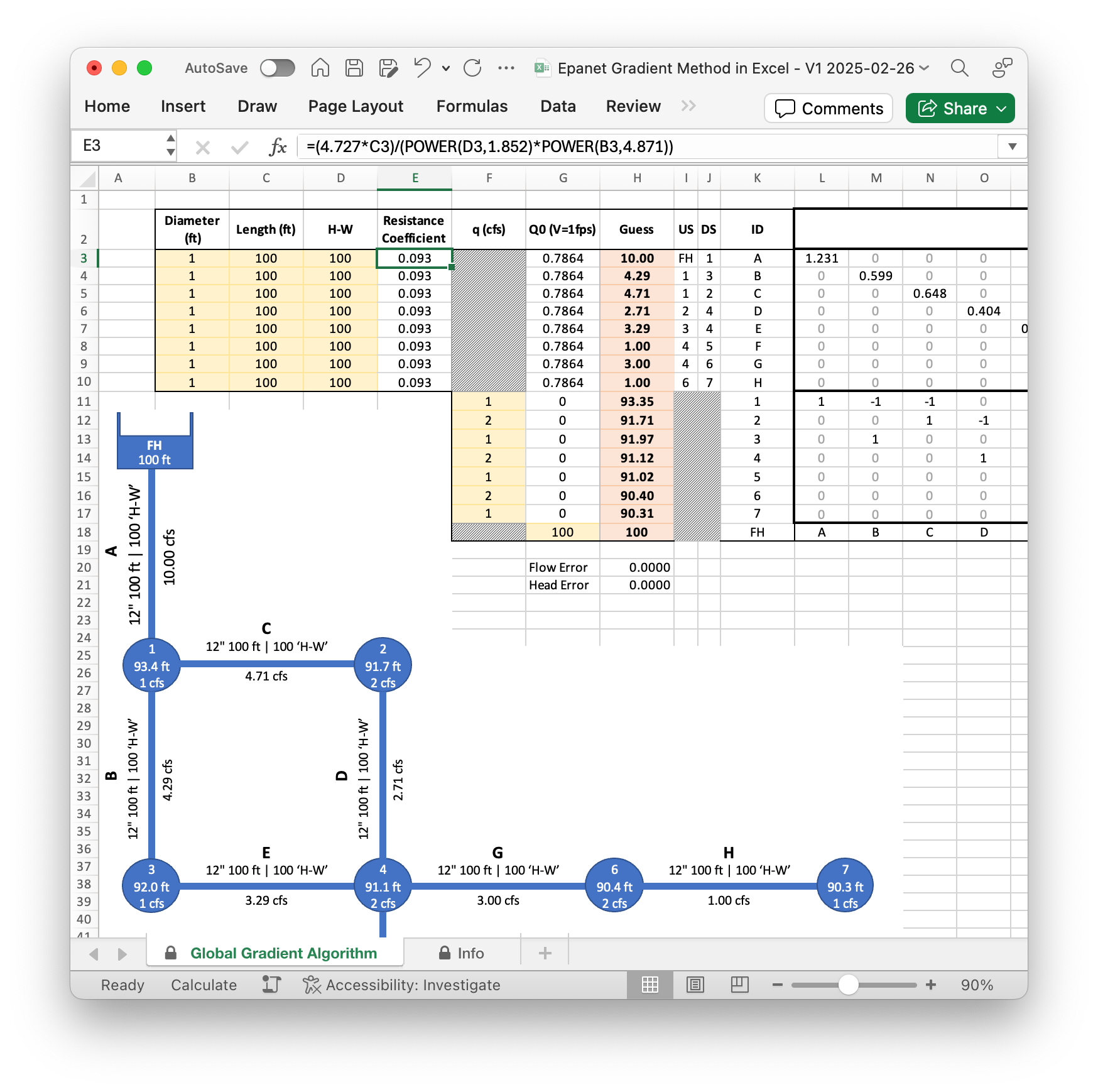
When I was doing research for my hydraulic modeling course, I wanted to better understand how EPANET works, so I recreated EPANET's algorithm inside Excel. You can download the Excel workbook below, but first, here’s a little background about why I created the workbook and why you might want to give it a try.

Why does understanding EPANET’s algorithm matter?

Under the hood, EPANET performs a complex algorithm to describe the flow of water through networks of pipes, pumps, and valves. That’s a good thing for us hydraulic modelers, because the nonlinear equations and the iterative nature of the solution process is far too impractical for humans to perform manually.

But with those calculations happening in the background, hydraulic modeling software can become like a black box. You don’t know why you’re getting the results you’re getting, and that can make you second-guess whether your model is up to par.

When you have a deeper understanding of how EPANET works, it can make it easier for you to:

1. Grasp underlying assumptions and limitations behind simulations.
2. Trust and feel more confident with EPANET results.
3. Identify, troubleshoot, and resolve modelling errors more easily.

If you’re not the biggest fan of complex mathematics, that’s ok. Academic papers explaining hydraulic modeling algorithms like Todini’s Global Gradient Algorithm or even EPANET’s algorithm backgrounder can be a little intimidating, or simply un-engaging. The Excel workbook at the end of this blog helps break the complexity down.

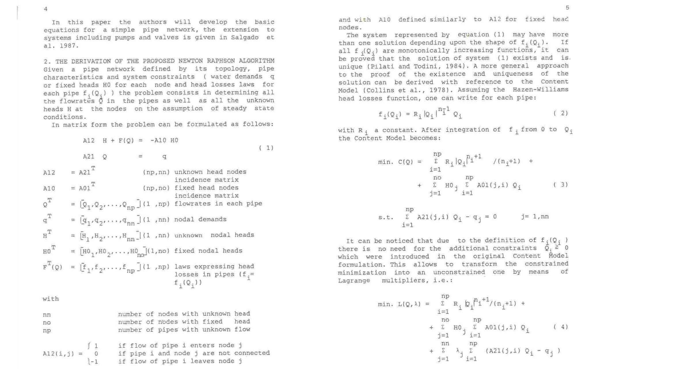
Todini, E., & Pilati, S. - A gradient algorithm for the analysis of pipe networks.

I prefer hands-on learning. That’s why Mark Wilson’s video on the Gradient Method was super helpful when I was exploring this topic. The Excel workbook is based on Mark’s video, but it uses a slightly different network. I plan to create my own video explaining the workbook, but in the meantime, be sure to check out Mark’s video.

The Gradient Algorithm

warning

The description below is a bit complicated. Don’t worry if you don’t get it in the first pass. Watch the videos, play with the excel spreadsheet, and reread this a few times, and it will start to piece together..

EPANET uses the Global Gradient Algorithm (GGA) to solve the complex set of equations that describe how water flows through distribution networks. These equations represent the interconnected nodes (junctions, reservoirs, tanks), links (pipes, pumps, valves), and their hydraulic properties (e.g., flow, pressure, head). The GGA is particularly effective in managing these nonlinear equations, which come from the relationship between flow and head loss in pipes, based on equations like Hazen-Williams and Darcy-Weisbach.

The GGA uses an iterative approach, based on the Newton-Raphson method, to adjust the flow rates and nodal heads within the network. This is done according to the laws of conservation of energy across links and conservation of mass in nodes. The algorithm begins with an initial estimate of the flow in each link (which may not necessarily satisfy flow continuity). Note that initially the value for junction heads are unknown. At each iteration of GGA:

1. A system of linear equations is solved to find nodal heads:

   a. Unlike early local approaches (Hardy-Cross) which dealt with one equation at the time, GGA deals directly with the system of non-linear equations describing the system hydraulic behaviour (Todini 2013).

   b. These equations involve the conservation of energy (non-linear equations), as described by Bernoulli’s principle applied across the length of each pipe, as well as conservation of mass (linear equations), which requires that total inflow equal total outflow at each network node to which pipes are connected.

   c. To solve this complex system of partly linear and partly non-linear equations, linearization of the non-linear equations is performed by means of the Newton Raphson gradient techniques, effectively reducing the problem to a system of linear equations (Todini 2006).

   d. The system of linear equations is solved and the new nodal heads are found.

2. The recently found nodal heads are used to estimate new flows:

   a. A correction term is computed to each pipe’s flow by taking into account the recently computed heads, as well as the pipe’s flow and headloss from previous iteration.

   b. New flows are obtained by updating the flow of each pipe (i.e., the flow of the previous iteration) according to the pipe’s specific correction term.

In short, GGA solves the problem of a nonlinear system of equations by iteratively solving a system of linear equations. The iterations continue until some suitable convergence criteria is met. Convergence criteria include the residual errors associated with the mass and energy conservation equations being below a certain predefined value, or the changes in flows become negligible.

An important note is that the convergence of the GGA is neither affected by the initial guess of an initial solution nor the complexity of the network (Todini 1988).

You can use Excel to step through each iteration and see how the flow rates and nodal heads are adjusted, gradually leading to a converged solution.

Download the Gradient Method in Excel

Download the Excel Workbook below to try it yourself. One of the nice things about this workbook is I’ve enabled circular references and repeating calculations, so Excel automatically finds the right answer and you don’t have to manually change the starting values for head and flow at each iteration.

That means you can update any of the parameters in the model, like demand at nodes or pipe properties, and see the results immediately. If it's not working for you, check if iterative calculations in Excel are enabled.

I hope you find that when you explore EPANET's algorithm through Excel, it not only demystifies complex hydraulic modeling processes but also empowers you with a deeper understanding and confidence in interpreting the result.

Todini, E., & Pilati, S. (1988). A gradient algorithm for the analysis of pipe networks. In Computer applications in water supply: vol. 1—systems analysis and simulation (pp. 1-20).

Todini, E. (2006). On the convergence properties of the different pipe network algorithms. In Water Distribution Systems Analysis Symposium 2006 (pp. 1-16).

Todini, E., & Rossman, L. A. (2013). Unified framework for deriving simultaneous equation algorithms for water distribution networks. Journal of Hydraulic Engineering, 139(5), 511-526.